Home > Teaching > Tutorials > R Tutorial Index
2 ::: Statistics with Data Frame Basics
variable information
tables of paired data
plots of paired data
When working in R, variables are often created. Basic information about a variable may be obtained in two ways: class and summary. If a variable vrb is a data frame (data that is imported is often in the form of a data frame), then we can look at the basic information about vrb:
> class(vrb)
[1] "data.frame"
> summary(vrb)
    Year         Gender           Farm
 Y1880: 750   Female:1019   Farm    : 201
 Y1990:1500   Male  :1231   Non-farm:2049
With a data frame (or a matrix), another function can be applied to find out the dimensions of the data:
> dim(vrb)
[1] 2250    3
2250 is the number of rows (usually observations) in the data and 3 is the number of columns available in the data.
If a variable is a vector (for example, vrb[ ,"Year"], which would be called "numeric" when inquiring about its class), the length function may be applied to find out its length:
> length(vrb[ ,"Year"])
[1] 2250
Tables are often useful for looking at paired data (such as Age and Gender of a group of people). Usually data in this form is found in a data frame. Suppose the data frame is called DF and DF has been attached (see the data frames section) and there are two variables of interest, Year and Gender. A table of the counts of each combination of the possible values is given by using table:
> table(Gender, Year)
        Year
Gender   Y1880 Y1990
  Female   280   739
  Male     470   761
If Gender and Year had been reversed in table, then the table would also be different (try it). If a table that gives proportions is of interest, the function prop.table may be applied to the table:
> tab1 <- table(Gender, Year)
> prop.table(tab1,1)
        Year
Gender       Y1880     Y1990
  Female 0.2747792 0.7252208
  Male   0.3818034 0.6181966
> tab2 <- prop.table(tab1,2)
> tab2
        Year
Gender       Y1880     Y1990
  Female 0.3733333 0.4926667
  Male   0.6266667 0.5073333
Notice how the second argument in the function changes whether the sums along the rows or columns will add to one. If only a couple decimal places are of interest, use the function round, where the second argument is the number of places after the decimal:
> round(tab2, 2)
        Year
Gender   Y1880 Y1990
  Female  0.37  0.49
  Male    0.63  0.51
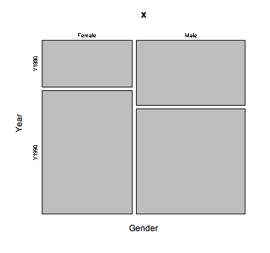
Plots of the data can be created by using either plot or barplot. For example,
> plot(tab1)

Color may be added by adding in a color argument into plot:
> plot(tab1, col=rainbow(4))

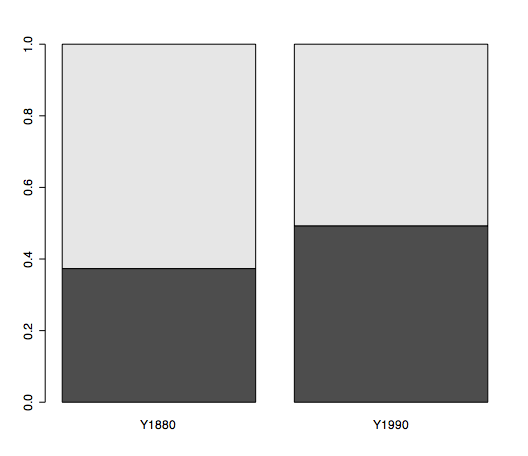
If a bar plot is of interest but the real interest is to compare proportions and how they change, then apply the function prop.table before applying the barplot function:
> barplot( prop.table(tab1,2) )
